Post 1 · Measure First

#

You cannot optimize what you haven’t measured — Low-Latency From The Ground Up

#

David Chan, Claude Opus 4.8 AI-Symbiosis Research · July 2026

The first rule of making something fast is that you are not allowed to guess. Not because guessing is lazy — because guessing is wrong, reliably, in a specific and humbling way. The human intuition for “where the time goes” is calibrated on reading code top to bottom, and code doesn’t execute in proportion to how much of it there is. So we start every optimization the same way: instrument, run, look.

The pipeline

#

The subject is real: Fortuna’s daily signal engine (lab11_signal_engine.py). Once a day it does four things per asset:

1. fetch        pull OHLC price history
2. indicators   rolling mean / std / z-score
3. fit_hmm      fit a Gaussian hidden-Markov regime model (Bull / Choppy / Bear)
4. db_write     log the signal row to SQLite

Then it decides ENTER / HOLD / EXIT / SKIP from the z-score and the regime. It’s a batch job on a cron, not an HFT engine — but the question “where does the time go?” has an answer regardless, and the way we find it is the whole skill.

Guess first (so the measurement can correct you)

#

Quick — before scrolling — which stage do you think dominates? Most people’s instinct lands on one of:

• “The fetch / data load — I/O is always the slow part.”
• “The SQLite writes — databases are slow.”
• “Fitting a machine-learning model, probably.”

Hold your guess. We’re going to take the network out of it (so the measurement is reproducible and network-jitter-free) and time the compute path on local BTC data — the CSV load standing in for the fetch. Everything else is the engine’s real code, unchanged.

The instrument

#

No fancy profiler yet — just the single most useful line in performance work, time.perf_counter(), wrapped around each stage:

def timed(fn, *a):
    t = time.perf_counter()
    out = fn(*a)
    return (time.perf_counter() - t) * 1000, out   # milliseconds

dt, raw = timed(load_raw)          # load CSV  (stands in for network fetch)
di, df  = timed(indicators, raw)   # rolling mean/std/z-score
dh, _   = timed(fit_hmm, df)       # the 10-restart Gaussian HMM
dw, _   = timed(db_write, rows)    # SQLite insert + commit

Run it 20 times and take the median (one run tells you nothing — you need a distribution to separate signal from scheduler noise). That’s it. That’s the whole tool. People reach for flame graphs before they’ve reached for this, and they shouldn’t.

The result

#

stage           median (ms)      p95       min       max    % of total
─────────────────────────────────────────────────────────────────────
load_csv            8.76        10.82      6.32     11.78       0.4 %
indicators          1.60         1.78      1.44      2.23       0.1 %
fit_hmm          2327.10      2428.47   2226.74   2438.92      99.5 %
db_write            0.69         0.78      0.48      0.79       0.0 %
─────────────────────────────────────────────────────────────────────
total            2338.71      2440.05

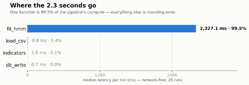
There it is. fit_hmm is 99.5% of the compute. Everything else — loading a 780 KB CSV, computing the indicators, writing to SQLite — sums to half a percent. The database you might have “optimized.” The data load you assumed was the bottleneck. Rounding error, all of it.

Visually, the pipeline is one bar:

Why this is the entire lesson

#

This is Amdahl’s law made concrete. The speedup available to you is capped by the fraction of time you’re actually able to touch. If I spent a heroic week making the SQLite writes 10× faster, I’d shave 0.6 ms off a 2,339 ms job — a 0.03% win for a week of work. If I make fit_hmm just 2× faster, I halve the whole pipeline. Same effort budget, a 1000× difference in payoff, and the only way to know which is which is the table above.

So the measurement didn’t just give me a number — it gave me a map of where I’m allowed to spend effort. Three of the four stages are now permanently off the table. That’s not a small result; that’s the result. Most wasted optimization work in the world is spent lovingly tuning the 0.5%.

Notice too what the distribution tells us: fit_hmm ranges 2227–2439 ms across runs — ~9% spread. That variance is itself a clue (non-determinism in the fit) that Post 2 will follow inside the function.

What we proved

#

• Guessing is out. Had I trusted intuition, “slow database” or “slow I/O” were the plausible-sounding wrong answers.
• One perf_counter and 20 runs beat any amount of staring at code.
• The hot path is fit_hmm, and nothing else is worth touching until it is.

The whole game from here is that one function. Next post, we go inside it: why does fitting a Gaussian HMM cost 2.3 seconds — and what, specifically, is burning the cycles?

Next — Post 2 · Anatomy of a Hot Path: ten random restarts, 200 EM iterations, full-covariance matrices. We profile the inside of fit_hmm and find the actual cycles before we touch a line of it.